Optimal control¶

The optimal module provides support for optimization-based controllers for nonlinear systems with state and input constraints.

Problem setup¶

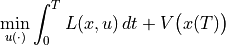
Consider the optimal control problem:

$\min_{u(\cdot)} \int_0^T L(x,u)\, dt + V \bigl( x(T) \bigr)$

subject to the constraint

$\dot x = f(x, u), \qquad x\in\mathbb{R}^n,\, u\in\mathbb{R}^m.$

Abstractly, this is a constrained optimization problem where we seek a feasible trajectory $(x(t), u(t))$ that minimizes the cost function

$J(x, u) = \int_0^T L(x, u)\, dt + V \bigl( x(T) \bigr).$

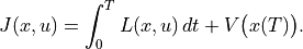
More formally, this problem is equivalent to the “standard” problem of minimizing a cost function $J(x, u)$ where $(x, u) \in L_2[0,T]$ (the set of square integrable functions) and $h(z) = \dot x(t) - f(x(t), u(t)) = 0$ models the dynamics. The term $L(x, u)$ is referred to as the integral (or trajectory) cost and $V(x(T))$ is the final (or terminal) cost.

It is often convenient to ask that the final value of the trajectory, denoted $x_\text{f}$ , be specified. We can do this by requiring that $x(T) = x_\text{f}$ or by using a more general form of constraint:

$\psi_i(x(T)) = 0, \qquad i = 1, \dots, q.$

The fully constrained case is obtained by setting $q = n$ and defining $\psi_i(x(T)) = x_i(T) - x_{i,\text{f}}$ . For a control problem with a full set of terminal constraints, $V(x(T))$ can be omitted (since its value is fixed).

Finally, we may wish to consider optimizations in which either the state or the inputs are constrained by a set of nonlinear functions of the form

$\text{lb}_i \leq g_i(x, u) \leq \text{ub}_i, \qquad i = 1, \dots, k.$

where $\text{lb}_i$ and $\text{ub}_i$ represent lower and upper bounds on the constraint function $g_i$ . Note that these constraints can be on the input, the state, or combinations of input and state, depending on the form of $g_i$ . Furthermore, these constraints are intended to hold at all instants in time along the trajectory.

A common use of optimization-based control techniques is the implementation of model predictive control (also called receding horizon control). In model predictive control, a finite horizon optimal control problem is solved, generating open-loop state and control trajectories. The resulting control trajectory is applied to the system for a fraction of the horizon length. This process is then repeated, resulting in a sampled data feedback law. This approach is illustrated in the following figure:

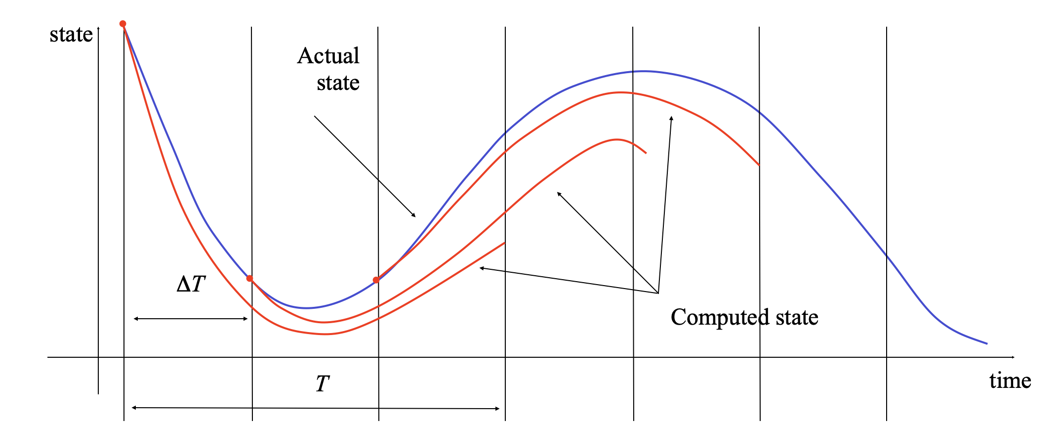
Every $\Delta T$ seconds, an optimal control problem is solved over a $T$ second horizon, starting from the current state. The first $\Delta T$ seconds of the optimal control $u_T^{\*}(\cdot; x(t))$ is then applied to the system. If we let $x_T^{\*}(\cdot; x(t))$ represent the optimal trajectory starting from $x(t)$ then the system state evolves from $x(t)$ at current time $t$ to $x_T^{*}(\delta T, x(t))$ at the next sample time $t + \Delta T$ , assuming no model uncertainty.

In reality, the system will not follow the predicted path exactly, so that the red (computed) and blue (actual) trajectories will diverge. We thus recompute the optimal path from the new state at time $t + \Delta T$ , extending our horizon by an additional $\Delta T$ units of time. This approach can be shown to generate stabilizing control laws under suitable conditions (see, for example, the FBS2e supplement on Optimization-Based Control.

Module usage¶

The optimal control module provides a means of computing optimal trajectories for nonlinear systems and implementing optimization-based controllers, including model predictive control. It follows the basic problem setup described above, but carries out all computations in discrete time (so that integrals become sums) and over a finite horizon. To local the optimal control modules, import control.optimal:

import control.optimal as obc

To describe an optimal control problem we need an input/output system, a time horizon, a cost function, and (optionally) a set of constraints on the state and/or input, either along the trajectory and at the terminal time. The optimal control module operates by converting the optimal control problem into a standard optimization problem that can be solved by scipy.optimize.minimize(). The optimal control problem can be solved by using the solve_ocp() function:

res = obc.solve_ocp(sys, timepts, X0, cost, constraints)

The sys parameter should be an InputOutputSystem and the timepts parameter should represent a time vector that gives the list of times at which the cost and constraints should be evaluated.

The cost function has call signature cost(t, x, u) and should return the (incremental) cost at the given time, state, and input. It will be evaluated at each point in the timepts vector. The terminal_cost parameter can be used to specify a cost function for the final point in the trajectory.

The constraints parameter is a list of constraints similar to that used by the scipy.optimize.minimize() function. Each constraint is specified using one of the following forms:

LinearConstraint(A, lb, ub)
NonlinearConstraint(f, lb, ub)

For a linear constraint, the 2D array A is multiplied by a vector consisting of the current state x and current input u stacked vertically, then compared with the upper and lower bound. This constraint is satisfied if

lb <= A @ np.hstack([x, u]) <= ub

A nonlinear constraint is satisfied if

lb <= f(x, u) <= ub

By default, constraints are taken to be trajectory constraints holding at all points on the trajectory. The terminal_constraint parameter can be used to specify a constraint that only holds at the final point of the trajectory.

The return value for solve_ocp() is a bundle object that has the following elements:

res.success: True if the optimization was successfully solved

res.inputs: optimal input

res.states: state trajectory (if return_x was True)

res.time: copy of the time timepts vector

In addition, the results from scipy.optimize.minimize() are also available.

To simplify the specification of cost functions and constraints, the ios module defines a number of utility functions:

`quadratic_cost`(sys, Q, R[, x0, u0])	Create quadratic cost function
`input_poly_constraint`(sys, A, b)	Create input constraint from polytope
`input_range_constraint`(sys, lb, ub)	Create input constraint from polytope
`output_poly_constraint`(sys, A, b)	Create output constraint from polytope
`output_range_constraint`(sys, lb, ub)	Create output constraint from range
`state_poly_constraint`(sys, A, b)	Create state constraint from polytope
`state_range_constraint`(sys, lb, ub)	Create state constraint from polytope

Example¶

Consider the vehicle steering example described in FBS2e. The dynamics of the system can be defined as a nonlinear input/output system using the following code:

import numpy as np
import control as ct
import control.optimal as opt
import matplotlib.pyplot as plt

def vehicle_update(t, x, u, params):
    # Get the parameters for the model
    l = params.get('wheelbase', 3.)         # vehicle wheelbase
    phimax = params.get('maxsteer', 0.5)    # max steering angle (rad)

    # Saturate the steering input
    phi = np.clip(u[1], -phimax, phimax)

    # Return the derivative of the state
    return np.array([
        np.cos(x[2]) * u[0],            # xdot = cos(theta) v
        np.sin(x[2]) * u[0],            # ydot = sin(theta) v
        (u[0] / l) * np.tan(phi)        # thdot = v/l tan(phi)
    ])

def vehicle_output(t, x, u, params):
    return x                            # return x, y, theta (full state)

# Define the vehicle steering dynamics as an input/output system
vehicle = ct.NonlinearIOSystem(
    vehicle_update, vehicle_output, states=3, name='vehicle',
    inputs=('v', 'phi'), outputs=('x', 'y', 'theta'))

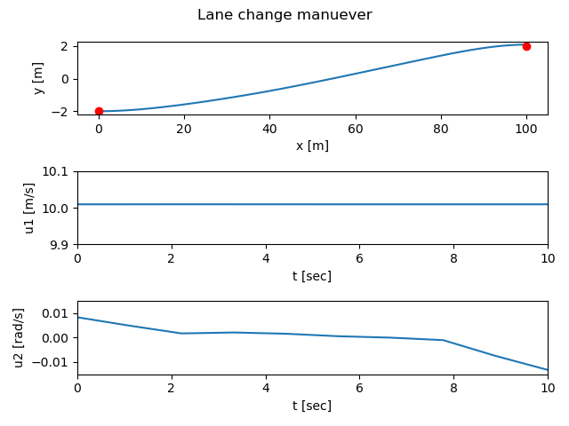
We consider an optimal control problem that consists of “changing lanes” by moving from the point x = 0 m, y = -2 m, $\theta$ = 0 to the point x = 100 m, y = 2 m, $\theta$ = 0) over a period of 10 seconds and with a with a starting and ending velocity of 10 m/s:

x0 = np.array([0., -2., 0.]); u0 = np.array([10., 0.])
xf = np.array([100., 2., 0.]); uf = np.array([10., 0.])
Tf = 10

To set up the optimal control problem we design a cost function that penalizes the state and input using quadratic cost functions:

Q = np.diag([0, 0, 0.1])          # don't turn too sharply
R = np.diag([1, 1])               # keep inputs small
P = np.diag([1000, 1000, 1000])   # get close to final point
traj_cost = opt.quadratic_cost(vehicle, Q, R, x0=xf, u0=uf)
term_cost = opt.quadratic_cost(vehicle, P, 0, x0=xf)

We also constraint the maximum turning rate to 0.1 radians (about 6 degees) and constrain the velocity to be in the range of 9 m/s to 11 m/s:

constraints = [ opt.input_range_constraint(vehicle, [8, -0.1], [12, 0.1]) ]

Finally, we solve for the optimal inputs:

timepts = np.linspace(0, Tf, 10, endpoint=True)
result = opt.solve_ocp(
    vehicle, timepts, x0, traj_cost, constraints,
    terminal_cost=term_cost, initial_guess=u0)

Plotting the results:

# Simulate the system dynamics (open loop)
resp = ct.input_output_response(
    vehicle, timepts, result.inputs, x0,
    t_eval=np.linspace(0, Tf, 100))
t, y, u = resp.time, resp.outputs, resp.inputs

plt.subplot(3, 1, 1)
plt.plot(y[0], y[1])
plt.plot(x0[0], x0[1], 'ro', xf[0], xf[1], 'ro')
plt.xlabel("x [m]")
plt.ylabel("y [m]")

plt.subplot(3, 1, 2)
plt.plot(t, u[0])
plt.axis([0, 10, 9.9, 10.1])
plt.xlabel("t [sec]")
plt.ylabel("u1 [m/s]")

plt.subplot(3, 1, 3)
plt.plot(t, u[1])
plt.axis([0, 10, -0.015, 0.015])
plt.xlabel("t [sec]")
plt.ylabel("u2 [rad/s]")

plt.suptitle("Lane change manuever")
plt.tight_layout()
plt.show()

yields

Optimization Tips¶

The python-control optimization module makes use of the SciPy optimization toolbox and it can sometimes be tricky to get the optimization to converge. If you are getting errors when solving optimal control problems or your solutions do not seem close to optimal, here are a few things to try:

The initial guess matters: providing a reasonable initial guess is often needed in order for the optimizer to find a good answer. For an optimal control problem that uses a larger terminal cost to get to a neighborhood of a final point, a straight line in the state space often works well.
Less is more: try using a smaller number of time points in your optimization. The default optimal control problem formulation uses the value of the inputs at each time point as a free variable and this can generate a large number of parameters quickly. Often you can find very good solutions with a small number of free variables (the example above uses 3 time points for 2 inputs, so a total of 6 optimization variables). Note that you can “resample” the optimal trajectory by running a simulation of the sytem and using the t_eval keyword in input_output_response (as done above).
Use a smooth basis: as an alternative to parameterizing the optimal control inputs using the value of the control at the listed time points, you can specify a set of basis functions using the basis keyword in solve_ocp() and then parameterize the controller by linear combination of the basis functions. The control.flatsys module defines several sets of basis functions that can be used.
Tweak the optimizer: by using the minimize_method, minimize_options, and minimize_kwargs keywords in solve_ocp(), you can choose the SciPy optimization function that you use and set many parameters. See scipy.optimize.minimize() for more information on the optimzers that are available and the options and keywords that they accept.
Walk before you run: try setting up a simpler version of the optimization, remove constraints or simplifying the cost to get a simple version of the problem working and then add complexity. Sometimes this can help you find the right set of options or identify situations in which you are being too aggressive in what your are trying to get the system to do.

See Optimal control for vehicle steeering (lane change) for some examples of different problem formulations.

Module classes and functions¶

`OptimalControlProblem`(sys, timepts, ...[, ...])	Description of a finite horizon, optimal control problem.
`OptimalControlResult`(ocp, res[, ...])	Result from solving an optimal control problem.

`solve_ocp`(sys, horizon, X0, cost[, ...])	Compute the solution to an optimal control problem
`create_mpc_iosystem`(sys, horizon, cost[, ...])	Create a model predictive I/O control system
`input_poly_constraint`(sys, A, b)	Create input constraint from polytope
`input_range_constraint`(sys, lb, ub)	Create input constraint from polytope
`output_poly_constraint`(sys, A, b)	Create output constraint from polytope
`output_range_constraint`(sys, lb, ub)	Create output constraint from range
`state_poly_constraint`(sys, A, b)	Create state constraint from polytope
`state_range_constraint`(sys, lb, ub)	Create state constraint from polytope